Finding duplicate places in your data
· First published on  iska.is (2018)
Dealing with duplicate places is a challenging task. If you look at standard ways of dealing with duplicates, they revolve around string similairty algorithms, like Levenshtein,  Jaccard, Jaro-Winkler and
 so-on.
There’s a general task of finding duplicate records in databases. That involves dealing with things at a different scale than traditional string comparision algorithms handle. Dealing with all potential matches pair-wise is going to be extremely slow. There is a class of hashing algorithms that are good at dealing with such tasks. They are known as LSH or Locality-sensitive hashing. LSH is a powerful technique with many cool applications - this article by Uber engineering is one such.
What all these methods have in common is that they are relatively stateless. This is not needed for string comparision or data duplication detection. They do not have any idea what part of a word provides more context, and what is not really useful. This causes some issues when we are dealing with duplicate places as you shall see.
Let’s look at a few examples of why this task is challenging:
| # | Place 1 | Place 2 | Reason |
|---|---|---|---|
| 0 | Emelina’s | Emelina’s Peruvian Restaurant | Large edit distance |
| 1 | Hillsdale Mall Levi’s Outlet | Hillsdale Mall Gap Outlet | High string similarity but these differ in key terms. |
| 2 | San Francisco Airport | San Francisco Airport Terminal - 1 | Nested places are hard. |
| 3 | Central Park | Central Park Cafe | In New York City, near Central Park, These may well be different. In most other places, they are almost certainly the same. |
To solve this problem, the engineers at  Facebook wrote an excellent paper -
 Deduplicating a Places Database. I’ve prototyped the algorithm outlined in a section in the paper and will walk you through some of the results I’ve seen.
To be more precise, this is the problem we are trying to solve:
Given two place names and , and an approximate geographical location containing both of them, determine if the two names can refer to the same entity.
The solution sketch to this problem has three main components.
The first is a novel generative language model for places that identifies the core of a place name.
For example in “Emelina’s” vs “Emelina’s Peruvian Restaurant”, it identifies “Emelina’s” as the core and “Peruvian”, “Restaurant” as the background words. More on this later.
The second component is a language model that incorporates the spatial context, e.g., the presence of nearby land- marks, parks, malls, airports, major streets and the current city.
The spatial model helps us with distinguishing “Hillsdale Mall Levi’s Outlet” from “Hillsdale Mall Gap Outlet” and matching/non-matching Central Park and Central Park Cafe.
The third component of our solution is a place name similarity measure based on our language models.
I’m only going to talk about the first part. I’ll try and write follow up posts for the others.
Approach for the Simple Name Model
Let’s build some intuition by starting with an example. Consider the set of to be:
- Philz Coffee
- Starbucks Coffee
- Philz
Our goal is to come up with core words for each of these words. The result should be:
- Philz
- Starbucks
- Philz
This is because Coffee is a “Background” word.
Let’s define:
- - set of all tokens/words in our .
- - Probability that token is a core word.
- - Probability that token is a background word.
- - Probability that token | , is a core word.
Algorithm
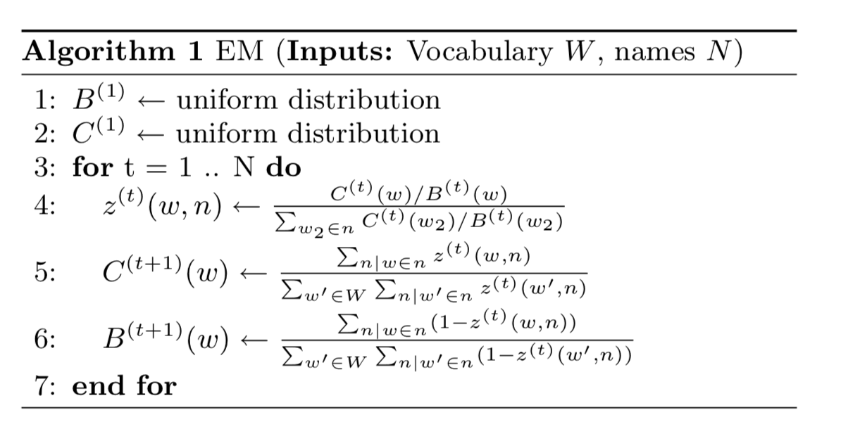
We start with . are uniform distributions. This looks like:
C[Philz] = C[Coffee] = C[Starbucks] = 1/3
B[Philz] = B[Coffee] = B[Starbucks] = 1/3
Thus, we have
- , and
Based on this, we will update our and values.
- and
If you notice, the core probability of Philz and the background probability of Coffee increases. The algorithm converges to the following solution:
The algorithm drives down the core probability of Coffee to 0 and background probabilities of Starbucks and Philz to 0.
eps = 1e-16

# this is to get map from token_number to word
def get_inverse_vocab_map(count_vect):
    invert = dict((v, k) for k, v in count_vect.vocabulary_.items())
    return collections.OrderedDict(sorted(invert.items()))


def compute_core_and_background(names, verbose=False):
    count_vect = CountVectorizer(stop_words='english', analyzer='word')
    word_vec = count_vect.fit_transform(names).toarray()

    invert = get_inverse_vocab_map(count_vect)
    w_T = word_vec.T

    n_words = len(count_vect.vocabulary_)
    n_names = len(names)

    C = np.full(n_words, 1.0 / n_words)
    B = np.full(n_words, 1.0 / n_words)

    Z = np.zeros((n_words, n_names))
    _round = 1

    while _round <= max(n_names, 100):
        _round += 1

        min_bg = np.min(B)
        # until convergence do us part
        if min_bg < eps:
            break

        amplified_coreness = C / B
        K = (w_T.T * amplified_coreness).T
        Z = K / np.sum(K, axis=0)
        C = np.sum(Z, axis=1) / np.sum(Z)
        Z_prime = w_T - Z
        B = np.sum(Z_prime, axis=1) / np.sum(Z_prime)

    # avoid division by zero
    B += eps

    if verbose:
        res = []
        for k, v in invert.items():
            k = (v, "core:", C[k], ", bg:", B[k])
            res.append(k)
        res.sort(key=lambda x: -(x[2] / x[-1]))
        for i in res:
            print(i)
    return count_vect, C, B
Let’s run this on our example:
_ = compute_core_and_background(
    ['Philz', 'Starbucks Coffee', 'Philz Coffee'], True)
('philz', 'core:', 0.6666666666666666, ', bg:', 1e-16)
('starbucks', 'core:', 0.3333333333333333, ', bg:', 1e-16)
('coffee', 'core:', 1.0087745832662039e-17, ', bg:', 1.0)Analyzing the points of interest in Palo Alto
For this exploration. I’m using the sample dataset of places in  Palo Alto, filtered to Zip Code: 94301.
Note: I’ve added some noise and duplicates to this dataset to make this effort more interesting.
palo_alto = pd.read_csv('https://gist.githubusercontent.com/iskakaushik/8a1c7580dd8f5ba2841bb009c28dbe76/raw/7d8aab8731e717bdbc388b1faa04af072ecb9798/palo-alto-places.csv')
names = palo_alto.name.tolist()

count_vect, C, B = compute_core_and_background(palo_alto.name.tolist())
palo_alto.head(3)| # | name | city | zip | latitude | longitude |
|---|---|---|---|---|---|
| 0 | wilby optical | palo alto | 94301 | 37.441920 | -122.141880 |
| 1 | deborahs palm | palo alto | 94301 | 37.450087 | -122.160125 |
| 2 | scandia home | palo alto | 94301 | 37.439012 | -122.159034 |
invert = get_inverse_vocab_map(count_vect)
core_word_identified = []

for name in names:
    one_hot_name = count_vect.transform([name]).toarray()[0]
    coreness_vector = one_hot_name * (C / B)
    hottest_i = np.argmax(coreness_vector)
    hotness_score = np.max(coreness_vector)
    core = invert[hottest_i]
    core_word_identified.append((core, name, hotness_score))

core_words_df = pd.DataFrame(core_word_identified, columns = ['core_word', 'name', 'score'])
core_words_df.head(3)| # | core_word | name | score |
|---|---|---|---|
| 0 | optical | wilby optical | 1.696486 |
| 1 | deborahs | deborahs palm | 1.696486 |
| 2 | scandia | scandia home | 1.696486 |
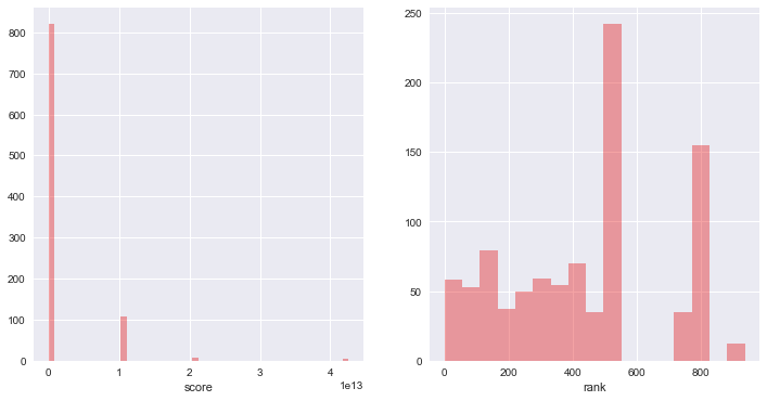
Score Distributions
Left is unscaled scores. Right ranks scores, to make the plot tighter.
Finding duplicates:
We identify the words that share the same core_word. We can tune the threshold to pick one that we are confident will result in strong matches. We can then deal with the duplicates by picking one or merging. We can use the score distribution to arrive at reasonable thresholds.
As you can see, we’ve identificed high condent matches.
THRESHOLD = 5.0

duplicates = core_words_df.groupby('core_word').filter(lambda x: len(x) >= 2).copy()
duplicates['rank'] = duplicates['score'].rank(method='min')
ranked_duplicates = duplicates.sort_values(by=['rank', 'core_word'], ascending=False)

high_score_ranked_dups = ranked_duplicates[ranked_duplicates.score > THRESHOLD]

print("%s high confident matches." % len(high_score_ranked_dups))

high_score_ranked_dups
22 high confident matches.| # | core_word | name | score | rank |
|---|---|---|---|---|
| 53 | coolsculpting | coolsculpting | 4.259851e+13 | 422.0 |
| 314 | coolsculpting | coolsculpting | 4.259851e+13 | 422.0 |
| 649 | coolsculpting | coolsculpting | 4.259851e+13 | 422.0 |
| 810 | coolsculpting | coolsculpting | 4.259851e+13 | 422.0 |
| 75 | walgreens | walgreens | 2.129925e+13 | 414.0 |
| 415 | walgreens | walgreens | 2.129925e+13 | 414.0 |
| 613 | kerastase | kerastase | 2.129925e+13 | 414.0 |
| 802 | kerastase | kerastase | 2.129925e+13 | 414.0 |
| 99 | cvs | cvs | 2.129925e+13 | 414.0 |
| 779 | cvs | cvs | 2.129925e+13 | 414.0 |
| 37 | chase | chase | 2.129925e+13 | 414.0 |
| 199 | chase | chase | 2.129925e+13 | 414.0 |
| 41 | mobile | spring mobile | 5.089457e+00 | 404.0 |
| 724 | mobile | t mobile | 5.089457e+00 | 404.0 |
| 475 | lemonade | lemonade la | 5.089457e+00 | 404.0 |
| 704 | lemonade | lemonade | 5.089457e+00 | 404.0 |
| 171 | footwear | tone footwear | 5.089457e+00 | 404.0 |
| 722 | footwear | footwear etc | 5.089457e+00 | 404.0 |
| 151 | comcast | comcast | 5.089457e+00 | 404.0 |
| 714 | comcast | comcast ventures | 5.089457e+00 | 404.0 |
| 454 | block | h and r block | 5.089457e+00 | 404.0 |
| 776 | block | block advisors | 5.089457e+00 | 404.0 |
Let’s take a look at some of the duplicates we have identified.
Not all duplicates are good
Here are some examples of matches on core words that had a low confidence score. Compare to . Art also lies in data exploration and picking the right thresholds.
| # | core_word | name | score | rank |
|---|---|---|---|---|
| 625 | alto | palo alto law horn and mantis kung fu | 0.561628 | 5.0 |
| 365 | alain | anna slutsky alain pinel realtors | 0.506742 | 3.0 |
| 788 | alain | alain pinel realtors | 0.506742 | 3.0 |
| 573 | service | a jag tax preparation and bookkeeping service | 0.481377 | 1.0 |
| 584 | service | gonzales juanita a ea tax preparation and bookkeeping service | 0.481377 | 1.0 |
Hope you had fun reading the post.
Thanks,
 Kaushik